MyD88^TIR small wedges¶

Introduction¶

The structures of MyD88^TIR domain higher-order assemblies were resolved by MicroED and SFX, providing insight into Toll-like receptor signal transduction. Details are published in this article:

MyD88 TIR domain higher-order assembly interactions revealed by microcrystal electron diffraction and serial femtosecond crystallography
Clabbers MTB, Holmes S, Muusse TW, Vajjhala PR, Thygesen SJ, Malde AK, Hunter DJB, Croll TI, Flueckiger L, Nanson JD, Rahaman MH, Aquila A, Hunter MS, Liang M, Yoon CH, Zhao J, Zatsepin NA, Abbey B, Sierecki E, Gambin Y, Stacey KJ, Darmanin C, Kobe B, Xu H, Ve T.
Nat Commun 12, 2578 (10 05 2021). [PMID:33972532] [PMC reprint: PMC8110528]

DIALS was not used during the original work, but the datasets have been made public. So we can show how to use DIALS to reproduce the published results.

Data¶

The datasets for this tutorial are available online at SBGrid:

Clabbers, MT.B., H Xu, and X Zou. 2021. “Microcrystal Electron Diffraction Data for: Myeloid Differentiation Primary Response Protein MyD88. PDB Code 7beq.” SBGrid Data Bank. 814.

The downloaded data consists of a directory with eighteen incrementally numbered subdirectories, 814/{1..18}, each of which contains diffraction images from a single crystal. We recommend doing data processing for each dataset in its own directory, separate from the images. For example, we can create a structure that mirrors the path to the images. From a BASH command prompt we can do that like this:

mkdir -p dials-proc/{1..18}

Exploratory analysis¶

Before we dive in and try to process all eighteen datasets we should perform some initial investigations to get a feel for the data and ensure the metadata describing the diffraction experiments is being read correctly. We might as well take the first dataset for this. To start, we change our working directory to our processing area, and then list the contents of the dataset directory.

cd dials-proc/1
ls ../../814/1

We see that dataset 1 consists of 72 images with the extension .img, with filenames numbered sequentially from 00001.img to 00072.img. If the DIALS programs are in the PATH we can now check if DIALS can interpret one of these images.

dials.show ../../814/1/00001.img

The output shows us that indeed DIALS recognises this image. Near the top of the output we see Format class: FormatSMVTimePix_SU_516x516, indicating that there is even a specific image reader for this image rather than DIALS falling back on a generic reader. That’s a good start, but if we look carefully through the rest of the output we might spot a problem.

Detector distance¶

distance: 2.193

Those with experience with DIALS might know that laboratory space distances in the program are measured in millimetres *. This is evident from an earlier line, pixel_size:{0.055,0.055} in which we see that the pixel size of the Timepix detector is 0.055 mm, i.e. 55 µm, as expected.

*: except for the wavelength, which is in Ångströms.

Here we see a general problem with the SMV file format used for these images. The format definition is not rigorous, so there is no way to be sure what units are in use. Despite that fact that almost all known SMV formats use millimetres for detector distance, this is not enforced by any standard, and we have clearly found an exception.

Let’s assume the distance should be 2193 millimetres and import the full dataset:

dials.import ../../814/1/*.img distance=2193

Looking at the metadata with dials.show show.imported.expt shows that the distance from the headers is now overwritten to be 2193 mm. Let’s now view the images:

dials.image_viewer imported.expt

There is a good description of functions available in the image viewer in other tutorials, such as Processing in Detail. Feel free to play with the settings. Nothing you do here will alter the experimental geometry or affect further processing.

We see from the position of the blue cross in the centre of the region of low angle scatter that the beam centre seems to be correctly recorded in the image headers.

Spot-finding¶

Finding appropriate spot-finding settings can be challenging for some electron diffraction datasets with commonly-used types of integrating detectors. However, in this case the Timepix is a counting detector with a gain of 1.0, avoiding issues with improperly-modelled detector response. The default spot-finding settings as used for X-ray photon counting detectors are also appropriate here. 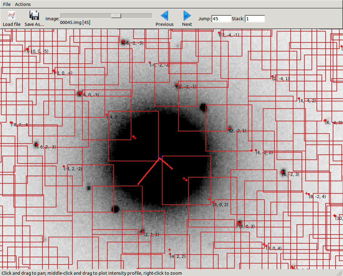We can view the effect of these settings in the dials.image_viewer. In this case we have ticked the box next to Threshold pixels in the Settings panel to show a diffraction image with the strong pixels marked up with a red overlay.

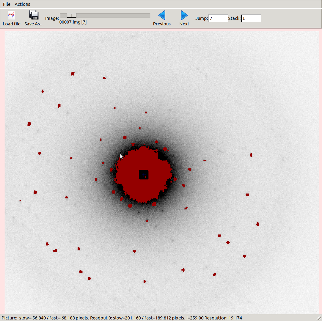
The strong diffraction spots are clearly being found, but we also see that a big region of inelastic scatter around the direct beam is picked up by the spot-finding algorithm. This might cause problems with indexing. By using the Resolution reading at the bottom of the image viewer we see that most of this occurs within a d-spacing of 20 Å or higher, so we’ll exclude that, but otherwise leave spot-finding settings as default:

dials.find_spots imported.expt d_max=20

The log shows the number of strong pixels found on each image, and then the number of spots these form, followed by how many make it through various filtering steps. The log ends with an ASCII-art histogram:

Histogram of per-image spot count for imageset 0:
633 spots found on 72 images (max 26 / bin)
                                    *
                                    *
    **                              *
    ***        * *  *   ** * *      **
    ***        * *  *  ***** *      **      *
    ***        * ** *  ***** * ** * ****  * *
    ***      *** ** * ****** * ** * ****  *** **    **   *
** ****     ****************** *****************  * ** * *
********  ************************************** **********
************************************************ ***********
1                          image                          72

--------------------------------------------------------------------------------

With X-ray datasets this histogram can often be used as a quick assessment of radiation damage. With electron diffraction that can be more difficult, both because the total rotation angle for the scan is usually smaller and because the Ewald sphere for electron diffraction is very flat. This means that the variability of this plot is rather high. Some orientations are close to zone axes and have many spots in the diffracting condition, whereas other orientations produce bands of fewer spots instead. We can explore the found spots now in the image viewer with this command:

dials.image_viewer imported.expt strong.refl

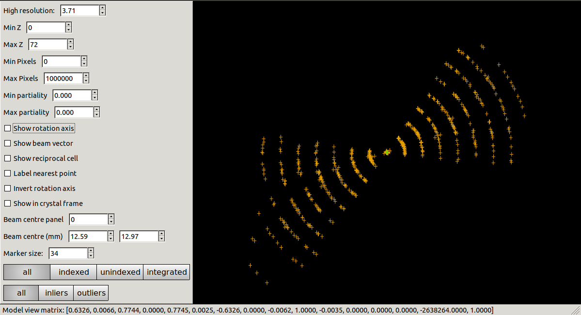
Another useful viewer is the 3D dials.reciprocal_lattice_viewer, which we will now launch like this

dials.reciprocal_lattice_viewer imported.expt strong.refl

But here we see a problem. The reciprocal lattice positions do not make a clean lattice. Here we have oriented the view down the putative rotation axis and instead of seeing separate spots we see arcs of points around that axis.

https://dials.github.io/images/MyD88/rlv-strong-wrong-axis.png

Tilt axis orientation¶

The diffraction geometry metadata printed by dials.show imported.expt suggests that the orientation of the rotation axis is given by

Rotation axis:   {0.782563,-0.622571,0}

But should we trust this? DIALS can search for the correct rotation axis like this:

dials.find_rotation_axis imported.expt strong.refl

This runs three levels of search: a global search, a local search and then a fine-search. The optimised rotation axis is written to a few file, optimised.expt and printed at the end of the log:

Rotation axis:   {-0.627963,-0.778243,0}

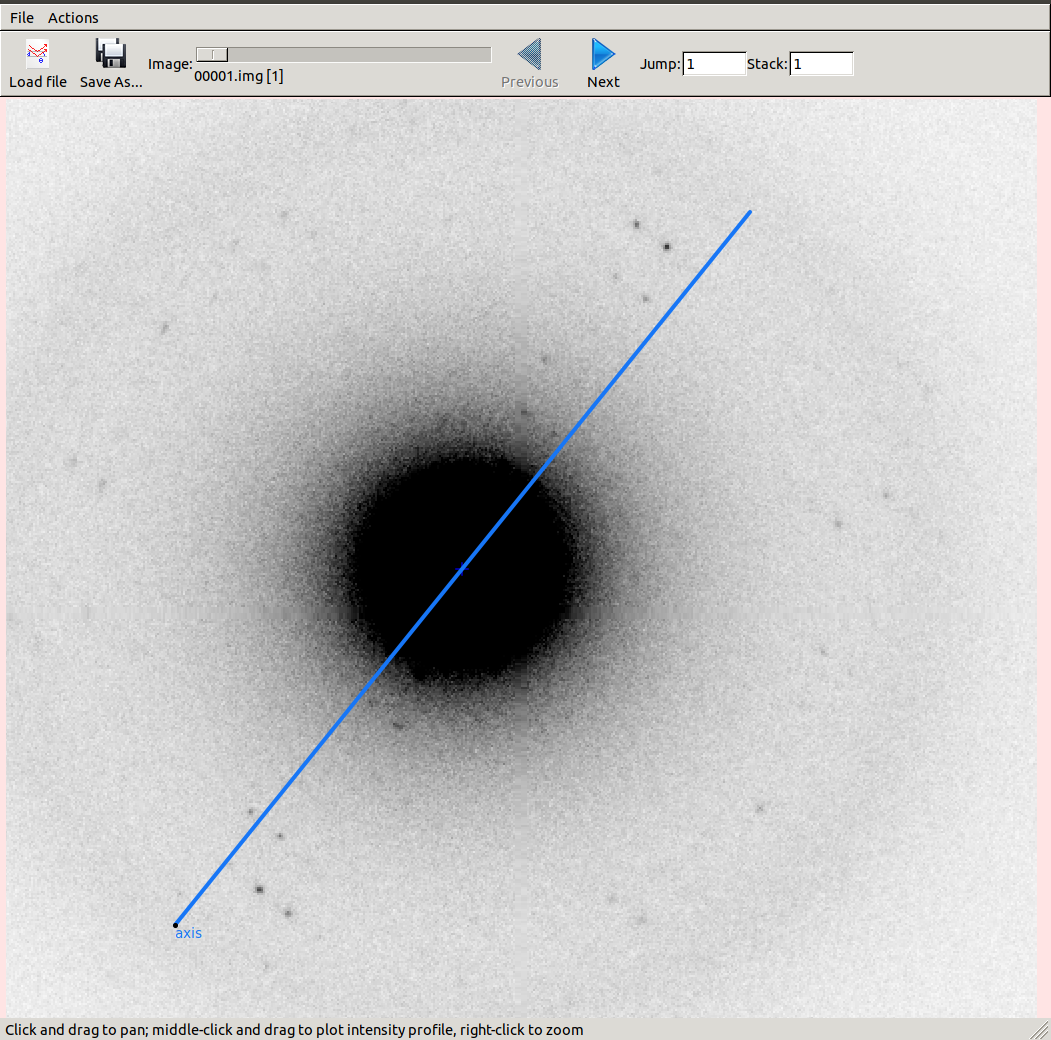
We can view the new rotation axis by opening optimised.expt in the image viewer and clicking on the “Rotation axis” checkbox.

https://dials.github.io/images/MyD88/rotation_axis.png

Now let’s view the reciprocal lattice:

dials.reciprocal_lattice_viewer optimised.expt strong.refl

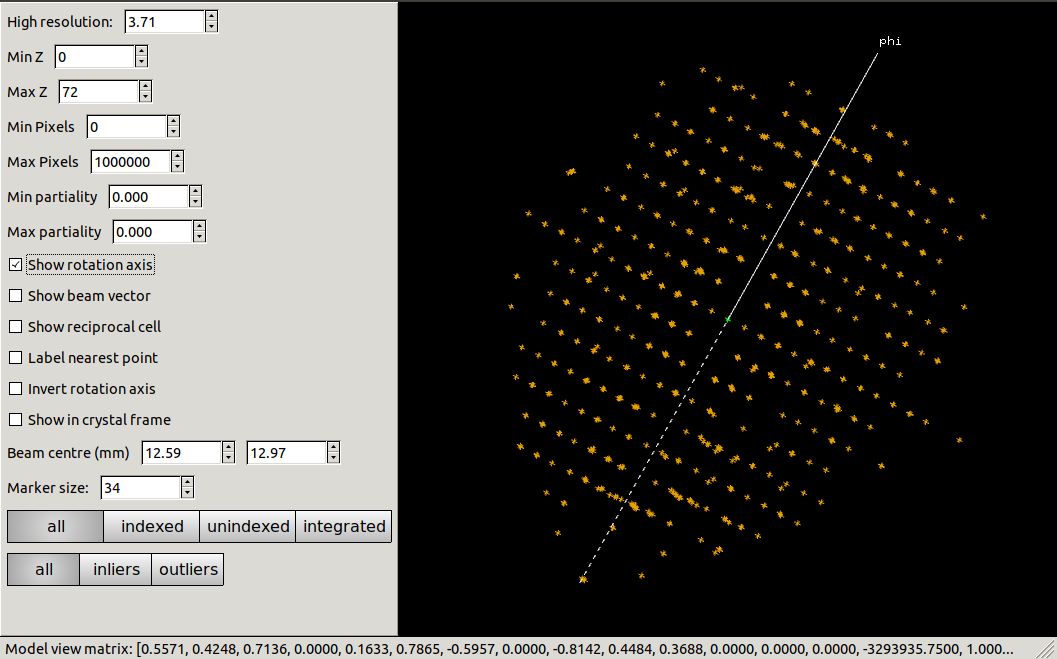
https://dials.github.io/images/MyD88/rlv-strong.png

Using the mouse we can rotate and zoom this view, and can easily find directions showing a well-ordered lattice. This gives us confidence that indexing will be successful.

Indexing¶

During indexing we will find a lattice and then refine the diffraction geometry to better fit the observed spots. One major difference between electron and X-ray diffraction is that the wavelength is much shorter (0.0251 Å in this case compared to ~1 Å typical for X-rays). As a result, the Ewald sphere is rather flat for electron diffraction and can be approximated by an “Ewald plane”. A side effect of this is that simultaneous refinement of the detector distance and the unit cell parameters is hardly possible. Changes in the distance can be offset by a scaling of the cell volume with negligible differences in the predicted spot positions. To avoid refinement wandering off to give unreasonable values for both the cell and distance, we typically fix the latter by adding the option detector.fix=distance to jobs that include geometry refinement. We will otherwise do indexing using the standard 3D FFT algorithm and other parameters as default, so the command we need is:

dials.index optimised.expt strong.refl detector.fix=distance

At the end of the log for this job we see a high proportion of indexed spots:

+------------+-------------+---------------+-------------+
|   Imageset |   # indexed |   # unindexed | % indexed   |
|------------+-------------+---------------+-------------|
|          0 |         562 |            70 | 88.9%       |
+------------+-------------+---------------+-------------+

and a little further up we see that the diffraction geometry model fits the observed spots quite nicely:

RMSDs by experiment:
+-------+--------+----------+----------+------------+
|   Exp |   Nref |   RMSD_X |   RMSD_Y |     RMSD_Z |
|    id |        |     (px) |     (px) |   (images) |
|-------+--------+----------+----------+------------|
|     0 |    528 |  0.51747 |  0.67141 |    0.28935 |
+-------+--------+----------+----------+------------+

The RMSDs are the root mean square deviation between observed and predicted spot positions for reflections used in refinement. The positional RMSDs are less than 1 pixel in both X (fast) and Y (slow) directions on the image and the RMSD in the tilt angle direction is less than 0.3 images.

Determining lattice symmetry¶

Unless a space group is explicitly specified, dials.index will return the best fitting triclinic (\(P\ 1\)) solution. A separate program, dials.refine_bravais_settings, can then be used to analyse the lattice symmetry and suggest a higher-symmetry point group. As this also does geometry refinement, we need to ensure the detector distance remains fixed:

dials.refine_bravais_settings indexed.expt indexed.refl detector.fix=distance

In the output we see two solutions: the original triclinic solution and a centred monoclinic lattice:

Chiral space groups corresponding to each Bravais lattice:
aP: P1
mI: I2
+------------+--------------+--------+--------------+----------+-----------+------------------------------------------+----------+--------------+
|   Solution |   Metric fit |   rmsd | min/max cc   |   #spots | lattice   | unit_cell                                |   volume | cb_op        |
|------------+--------------+--------+--------------+----------+-----------+------------------------------------------+----------+--------------|
|   *      2 |       1.4508 |  0.118 | 0.953/0.953  |      533 | mI        | 64.31  37.02 115.99  90.00 104.37  90.00 |   267504 | c,a,-a+2*b-c |
|   *      1 |       0      |  0.047 | -/-          |      528 | aP        | 37.07  61.63  64.40  72.88  89.25  73.45 |   134383 | a,b,c        |
+------------+--------------+--------+--------------+----------+-----------+------------------------------------------+----------+--------------+
* = recommended solution

If we knew nothing about the crystal structure beforehand we might continue and process with this solution. However, here we are going to “cheat” slightly and look at the cell from the published paper. There it is given as

Cell dimensions

a, b, c (Å)

99.06, 31.01, 54.30

α, β, γ (°)

90.00, 107.70, 90.00

Clearly we have found a different cell! There are two issues. The first is that dials.refine_bravais_settings selects the \(I\ 2\) setting here because by default, following standard practice, it favours monoclinic centred cells that have β angles closer to 90°. To compare our solution with the published \(C\ 2\) cell we can change that behaviour and run again:

dials.refine_bravais_settings indexed.expt indexed.refl detector.fix=distance best_monoclinic_beta=False

and with that we get

Chiral space groups corresponding to each Bravais lattice:
aP: P1
mC: C2
+------------+--------------+--------+--------------+----------+-----------+-------------------------------------------+----------+-----------+
|   Solution |   Metric fit |   rmsd | min/max cc   |   #spots | lattice   | unit_cell                                 |   volume | cb_op     |
|------------+--------------+--------+--------------+----------+-----------+-------------------------------------------+----------+-----------|
|   *      2 |       1.4508 |  0.118 | 0.953/0.953  |      533 | mC        | 117.84  37.02  64.31  90.00 107.54  90.00 |   267504 | a-2*b,a,c |
|   *      1 |       0      |  0.047 | -/-          |      528 | aP        | 37.07  61.63  64.40  72.88  89.25  73.45  |   134383 | a,b,c     |
+------------+--------------+--------+--------------+----------+-----------+-------------------------------------------+----------+-----------+
* = recommended solution

Now at least the β angle is about what we expect! However, the a, b and c axes are all a bit too long. In fact, they are all about 20% higher than the published values. The cell volume is too large. At the introduction to Indexing we noted that the cell volume and detector distance are highly correlated. It looks like the presumed detector distance of 2193 mm is still not correct.

We will fix that in the next section, but first we have to reindex the reflections to match the chosen Bravais lattice solution, bravais_setting_2.expt. To do that we take the change-of-basis operator from the solution table and pass that into the dials.reindex program:

dials.reindex indexed.refl change_of_basis_op=a-2*b,a,c

This creates a file reindexed.refl that is compatible with our chosen solution bravais_setting_2.expt.

Refining the detector distance¶

In situations where the correct unit cell is known it is possible to refine the detector distance. We can do this by providing a restraint to the known unit cell. This allows refinement of the unit cell and detector parameters simultaneously, while pushing the cell towards its ideal values, thus breaking the degeneracy between these parameters. The strength of this “push” is adjustable, so we have control over how much we want the data or the external target to affect the refined unit cell values.

To set up a restraint we must write a file using PHIL syntax. The interface to restraints is a bit awkward, but having written this once, we can then copy-and-paste it for other uses, with changes required only to the values and the sigmas. So, in a text editor, copy these lines and save the file as restraint.phil:

refinement
{
  parameterisation
  {
    crystal
    {
      unit_cell
      {
        restraints
        {
          tie_to_target
          {
            values=99.06,31.01,54.30,90,107.7,90
            sigmas=0.01,0.01,0.01,0.01,0.01,0.01
          }
        }
      }
    }
  }
}

This describes a restraint to the known cell with reasonably strong ties, given by fairly low sigma values.

The detector distance is defined as the distance along the most direct line to the sample, so it is also affected by “tilt” and “twist” orientation angles. These are rather poorly-defined by the positions of diffraction spots, so while we want the detector distance to refine, we choose to constraint the orientation (rotational) parameters for the detector.

dials.refine bravais_setting_2.expt reindexed.refl restraint.phil\
  detector.fix=orientation scan_varying=False

We added scan_varying=False to ensure that only “scan static” refinement is performed, otherwise we get one round of scan static refinement followed by a round of scan-varying refinement. The latter allows the crystal parameters to vary across the scan, but those smoothly-changing parameters are not affected by the restraint. In this situation, we are not trying to get a sophisticated, varying model for the diffraction geometry, but are just trying to correct the wrong detector distance.

At the end of the log we see that the unit cell now looks more like what we expect:

Final refined crystal model:
Crystal:
    Unit cell: 99.04(4), 31.09(2), 54.29(4), 90.0, 107.71(4), 90.0
    Space group: C 1 2 1

and the RMSDs still look reasonably good, so refinement appears to have been successful. We can see the new detector distance by showing the output experiments file:

dials.show refined.expt

which contains the line:

distance: 1843.57

Note

It would be prudent to repeat this procedure with all 18 datasets, but for the purposes of this tutorial we will take this value and assume it is appropriate for the other data sets. In general, it is much preferred if the detector distance is properly calibrated and stored along with the diffraction images!

We can now return to import with the correct detector distance and the rotation axis orientation, followed by the other steps to get back to the correctly indexed cell. We will skip the dials.refine_bravais_settings and dials.reindex steps now that we have determined the lattice symmetry, by selecting space_group=C2 during the indexing job. This will make it easier to script these steps for the other datasets.

dials.import ../../814/1/*.img distance=1843.57 goniometer.axis=-0.627963,-0.778243,0
dials.find_spots imported.expt d_max=20
dials.index imported.expt strong.refl detector.fix=distance\
  space_group=C2 output.experiments=C2.expt output.reflections=C2.refl

Integration¶

Now we have a suitable model for the experiment, we can go ahead and integrate the reflections. We won’t use any special options here.

dials.integrate refined.expt refined.refl

There is a table of output at the end of the log that provides some insight into how well this proceeded. In particular, if there are very large numbers of reflections that failed to integrate by either summation integration or profile fitting then we should investigate. In this case though, everything looks okay.

+---------------------------------------+-----------+--------+--------+
| Item                                  |   Overall |    Low |   High |
|---------------------------------------+-----------+--------+--------|
| dmin                                  |      2.12 |   5.76 |   2.12 |
| dmax                                  |     47.23 |  47.23 |   2.16 |
| number fully recorded                 |   4328    | 540    |   9    |
| number partially recorded             |    950    | 111    |   2    |
| number with invalid background pixels |    993    |   0    |  11    |
| number with invalid foreground pixels |    403    |   0    |  11    |
| number with overloaded pixels         |      0    |   0    |   0    |
| number in powder rings                |      0    |   0    |   0    |
| number processed with summation       |   4849    | 643    |   0    |
| number processed with profile fitting |   4917    | 631    |   2    |
| number failed in background modelling |      0    |   0    |   0    |
| number failed in summation            |    403    |   0    |  11    |
| number failed in profile fitting      |    335    |  12    |   9    |
| ibg                                   |     35.73 |  94.97 |  13.84 |
| i/sigi (summation)                    |      3.94 |  18.54 |   0    |
| i/sigi (profile fitting)              |      5.98 |  25.45 |   0    |
| cc prf                                |      0.99 |   0.99 |   0.99 |
| cc_pearson sum/prf                    |      0.99 |   0.99 |   0    |
| cc_spearman sum/prf                   |      0.77 |   0.92 |   0    |
+---------------------------------------+-----------+--------+--------+

We can open the integration results in the image viewer, showing how well the reflections are centred in their integration boxes.

dials.image_viewer integrated.expt integrated.refl

https://dials.github.io/images/MyD88/integration_shoeboxes.png

Here we see that the fairly large rocking curve for the reflections means there are many overlapping shoeboxes. However, this is fine as long as the peak regions do not overlap. We cannot easily see this here, but the limited number of failed profile fits tells us the peak regions are well separated. The size of the reflection shoebox model is given towards the top of dials.integrate.log:

Using 454 / 455 reflections for sigma calculation
Calculating E.S.D Beam Divergence.
Calculating E.S.D Reflecting Range (mosaicity).
 sigma b: 0.003907 degrees
 sigma m: 1.083698 degrees

At this stage we would learn much more about the quality of the data from scaling and merging. However this single dataset is very incomplete. We should try integrating all the other datasets first and including them in the scaling job.

Scripted processing¶

During the Exploratory analysis we came up with a reasonable set of processing commands for dataset 1, while figuring out incorrect or missing diffraction geometry metadata such as the detector distance and the rotation axis orientation and direction. Rather than repeat all those steps manually for the remaining datasets we will write a script to process them all in the same way. This example uses a BASH shell script on Linux, but we could do similar on other systems.

First we change to the directory above where we have been working on dataset 1, and if not already done, we’ll make separate processing directories for all the datasets

cd ..
mkdir -p {1..18}

Now we’ll use a text editor to make a file, called process.sh for example, and enter these lines:

#!/bin/bash
set -e
for i in {1..18}
do
  cd "$i"

  dials.import ../../814/"$i"/*.img goniometer.axis=-0.627963,-0.778243,0 distance=1843.57
  dials.find_spots imported.expt d_max=20 d_min=2.5
  dials.index imported.expt strong.refl detector.fix=distance goniometer.fix=None space_group=C2
  dials.refine indexed.expt indexed.refl detector.fix=distance
  dials.plot_scan_varying_model refined.expt
  dials.integrate refined.expt refined.refl prediction.d_min=2.5

  cd ..
done

Note we made a change compared to the processing instructions above for the first dataset. Because we determined the rotation axis only for that dataset, it might not be exactly right for all datasets in general. By adding the option goniometer.fix=None to the dials.index we allow optimisation of the rotation axis during diffraction geometry refinement. We now make this script executable and run it like this:

chmod +x process.sh
./process.sh

This should run through to completion (set -e ensures that it will stop if any one of the jobs fails with an error) and produce 18 integrated datasets.

Scaling¶

We now want to combine the 18 datasets, scale them together, and calculate merging statistics. We will use dials.scale for this. A particularly helpful feature of this program is its capability to automatically filter out bad parts of the combined dataset using the ΔCC½ metric. By default this removes complete datasets, which is useful for snapshot and small wedge serial crystallography where we tend to consider each dataset a unit and are not paying much attention to changes within each dataset caused, for example, by radiation damage. By contrast, in this case, we’d like to try filtering individual bad images rather than complete datasets.

Also, dials.scale optimises the error model using reflections with an expected intensity above a particular value. For synchrotron X-ray datasets the default of 25.0 seems to work fine, but in this case that results in rather few reflections being used for error modelling in the the low resolution shells, so we will decrease that value to 10.0.

mkdir -p scale
cd scale

dials.scale ../{1..18}/integrated.{expt,refl}\
  filtering.method=deltacchalf\
  deltacchalf.mode=image_group\
  deltacchalf.group_size=1\
  min_Ih=10.0\
  d_max=35\
  d_min=3.0

cd ..

The first three options passed to dials.scale set up the ΔCC½ filtering, in image_group mode rather than the default dataset, and we also set the group_size to 1 rather than the default 10 as these datasets are rather wide-sliced. We then set the error modelling inclusion cut-off, as explained above. Finally we set resolution limits. The low resolution cut-off of 35 Å was chosen to remove the lowest angle reflections in the region of high inelastic scatter, while the high resolution limit of 3.0 Å was chosen to match the processing published in the paper.

There are many options to explore in scaling, and no claim is made here that this job is optimal! There is still much to be learned regarding the best handling of 3DED data.

At the end of the dials.scale.log we see a table summarising the merging statistics:

                                             Overall    Low     High
High resolution limit                           3.00    8.10    3.00
Low resolution limit                           31.17   31.18    3.05
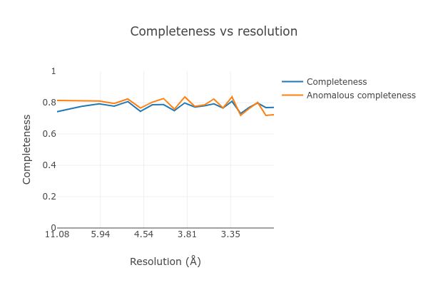
Completeness                                   77.5    74.2    77.0
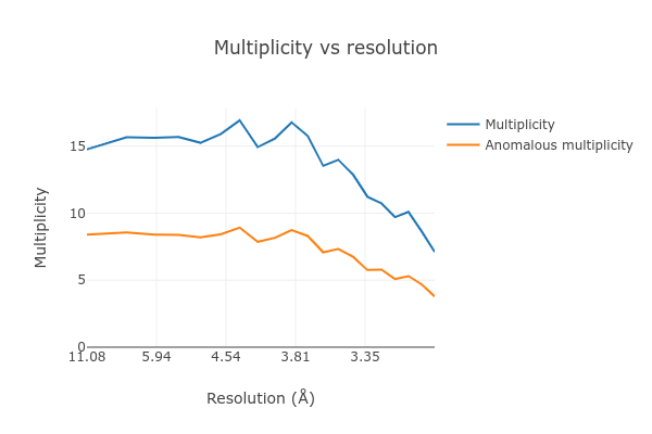
Multiplicity                                   13.6    14.8     7.1
I/sigma                                         6.9    12.9     1.9
Rmerge(I)                                     0.435   0.317   1.746
Rmerge(I+/-)                                  0.429   0.317   1.637
Rmeas(I)                                      0.452   0.328   1.886
Rmeas(I+/-)                                   0.460   0.336   1.830
Rpim(I)                                       0.113   0.080   0.657
Rpim(I+/-)                                    0.154   0.106   0.787
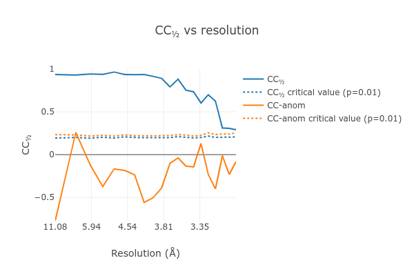
CC half                                       0.919   0.936   0.291
Anomalous completeness                         78.7    81.3    72.3
Anomalous multiplicity                          7.2     8.4     3.8
Anomalous correlation                        -0.419  -0.773  -0.082
Anomalous slope                               1.015
dF/F                                          0.173
dI/s(dI)                                      0.811
Total observations                            36662    2125     974
Total unique                                   2705     144     137

These, and many more, details are also saved to a HTML format report page. On Linux you can usually open this up with the command

xdg-open scale/dials.scale.html

This contains many useful plots, for example various statistics as a function of resolution:

https://dials.github.io/images/MyD88/cchalf.png

https://dials.github.io/images/MyD88/ioversigi.png

https://dials.github.io/images/MyD88/completeness.png

https://dials.github.io/images/MyD88/multiplicity.png

Further processing¶

Now we have processed the 18 datasets we want to export the data for structure solution and refinement. We can export the unmerged but scaled intensities in MTZ format (scaled.mtz) like this

dials.export scale/scaled.expt scale/scaled.refl

However, many downstream steps require the merged intensities, which we can create using the dials.merge program.

dials.merge scale/scaled.expt scale/scaled.refl

This creates the file merged.mtz, which we can use for structure solution by molecular replacement.

Cell dimensions
a, b, c (Å)	99.06, 31.01, 54.30
α, β, γ (°)	90.00, 107.70, 90.00

MyD88TIR small wedges¶