
Please click here to go to the tutorial for DIALS 2.2.
Small-molecule data reduction tutorial
Introduction
While the conventional use of DIALS for small molecule data could be to run xia2, the interactive processing steps via the command line are relatively straightforward. The aim of this tutorial is to step through the process…
Data
The data for this tutorial are on Zenodo at https://zenodo.org/record/51405 — we will use l-cyst_0[1-4].tar.gz i.e. the first four files. For this tutorial it will be assumed you have the data linked to a directory ../data — however this only matters for the import step.
Import
Usually DIALS processing is run on a sequence-by-sequence basis. For small molecule data however where multiple sequences from one sample are routinely collected, with different experimental configurations, it is helpful to process all sequences at once, therefore starting with:
dials.import ../data/*cbf
This will create a DIALS imported.expt file with details of the 4 sequences within it.
Spot finding
This is identical to the routine usage i.e.
dials.find_spots imported.expt nproc=8
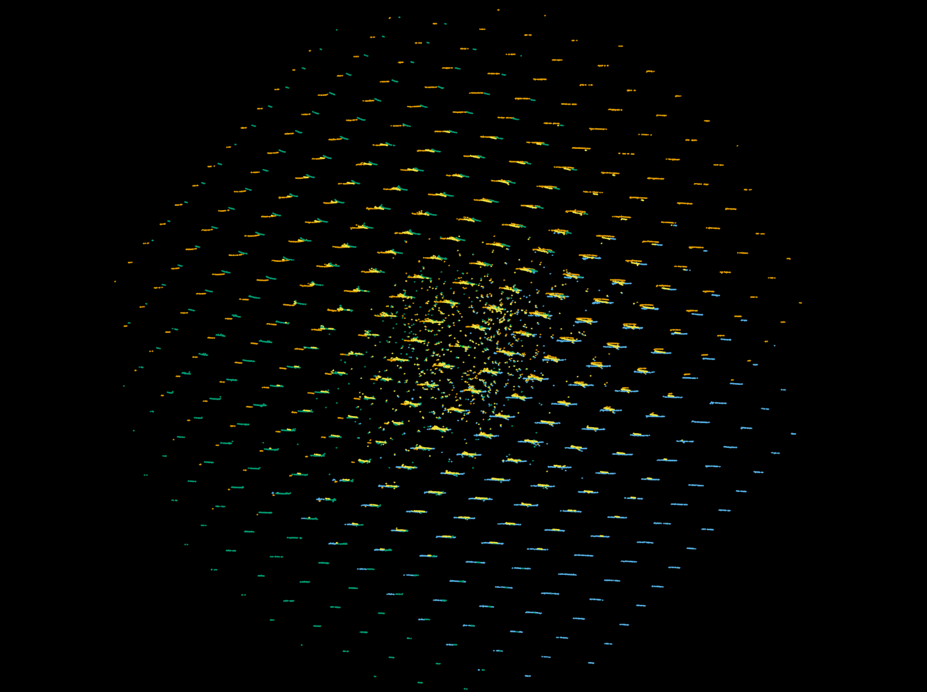
Though will of course take a little longer to work through four sequences. Here nproc=8 was assigned (for a core i7 machine.) The spot finding is independent from sequence to sequence but the spots from all sequences may be viewed with
dials.reciprocal_lattice_viewer imported.expt strong.refl
Which will show how the four sequences overlap in reciprocal space, as:
Indexing
Indexing here will depend on the model for the experiment being reasonably accurate. Provided that the lattices overlap in the reciprocal lattice view above, the indexing should be straightforward and will guarantee that all lattices are consistently indexed. One detail here is to split the experiments on output. This duplicates the models for the individual components rather than sharing them, which allows greater flexibility in refinement (and is critical for scan varying refinement).
dials.index imported.expt strong.refl
Without any additional input, the indexing will determine the most approproiate primitive lattice parameters and orientation which desctibe the observed reciprocal lattice positions.
Bravais lattice determination
In the single sequence tutorial the determination of the Bravais lattice is performed between indexing and refinement. This step however will only work on a single lattice at a time. Therefore in this case the analysis will be performed, the results verified then the conclusion fed back into indexing as follows:
dials.refine_bravais_settings indexed.refl indexed.expt crystal_id=0
dials.refine_bravais_settings indexed.refl indexed.expt crystal_id=1
dials.refine_bravais_settings indexed.refl indexed.expt crystal_id=2
dials.refine_bravais_settings indexed.refl indexed.expt crystal_id=3
Inspect the results, conclude that the oP lattice is appropriate then assign this as a space group for indexing (in this case, P222)
dials.index imported.expt strong.refl space_group=P222
This will once again consistently index the data, this time enforcing the lattice constraints.
Refinement
Prior to integration we want to refine the experimental geometry and the scan varying crystal orientation and unit cell. This is performed in two steps — the first is to perform static refinement on each indexed sequence, the second to take this refined model and refine the unit cell and orientation allowing for time varying parameters:
dials.refine indexed.refl indexed.expt output.reflections=static.refl output.experiments=static.expt scan_varying=false
dials.refine static.refl static.expt scan_varying=True
At this stage the reciprocal lattice view will show a much improved level of agreement between the indexed reflections from the four sequences:
dials.reciprocal_lattice_viewer refined.expt refined.refl
Integration
At this stage the reflections may be integrated. This is done by running
dials.integrate refined.refl refined.expt nproc=8
which will integrate each sequence in sequence, again using 8 cores.
Unit cell refinement
After integration the unit cell for downstream analysis may be derived from refinement of the cell against observed two-theta angles from the reflections, across the four sequences:
dials.two_theta_refine integrated.refl integrated.expt p4p=integrated.p4p
Here the results will be output to a p4p file for XPREP, which includes the standard uncertainties on the unit cell.
Output
After integration, the data should be split before exporting to a format suitable for input to XPREP or SADABS. Note that SADABS requires the batches and file names to be numbered from 1:
dials.split_experiments integrated.refl integrated.expt
dials.export format=sadabs reflections_0.refl experiments_0.expt sadabs.hklout=integrated_1.sad run=1
dials.export format=sadabs reflections_1.refl experiments_1.expt sadabs.hklout=integrated_2.sad run=2
dials.export format=sadabs reflections_2.refl experiments_2.expt sadabs.hklout=integrated_3.sad run=3
dials.export format=sadabs reflections_3.refl experiments_3.expt sadabs.hklout=integrated_4.sad run=4
If desired, p4p files for each combination of reflections_[0-3].refl, experiments_[0-3].expt could also be generated.