Lysozyme nanocrystals

Introduction

DIALS has been successfully adapted for processing electron diffraction data from protein nanocrystals. Extensions to the software and protocols for dealing with the peculiarities of electron diffraction data are described in a publication:

Electron diffraction data processing with DIALS

Clabbers MTB, Gruene T, Parkhurst JM, Abrahams JP, Waterman DG.

Acta Crystallogr D Struct Biol 74, 506-518 (01 06 2018). [PMID:29872002] [PMC reprint: PMC6096487]

Warning

This tutorial reproduces the data processing results described in that paper, which were produced by DIALS version 1.dev.2084-g06727c3 and CCP4 version 7.0.051. Results may differ with other versions of the software.

The commands listed here assume the use of a Bash shell on a POSIX-compliant system, so would have to be adjusted appropriately for use on other systems such as Windows.

Data

The data for this tutorial are available online at . There are seven datasets from different lysozyme nanocrystals stored as gzipped tar archives. These should be downloaded and expanded to create seven directories containing the images, Lys_ED_Dataset_{1..7}. We recommend doing data processing for each dataset in its own directory, separate from the images, for example Lys_ED_Dataset_1-dials-proc. When referring to the data directories in commands listed in this tutorial, we shall use an environment variable pointing to the parent directory. Assuming the current directory contains all of the downloaded and unpacked dataset directories, we set that variable as follows in a bash shell:

export DATA_PARENT=$(pwd)

Import

The images are in the standard miniCBF format, however the detector is unusual. We have constructed a special dxtbx Format class to interpret the images properly. This is not distributed with DIALS, but can be found in a separate repository here: https://github.com/dials/dxtbx_ED_formats.

We can make use of the dxtbx runtime plug-in system to pick the format class up automatically by saving it in a special directory, $HOME/.dxtbx/ (for POSIX-compliant systems). For example (may require installation of curl):

if [ ! -f ~/.dxtbx/FormatCBFMiniTimepix.py ]; then
  mkdir -p ~/.dxtbx
  curl -o ~/.dxtbx/FormatCBFMiniTimepix.py https://raw.githubusercontent.com/dials/dxtbx_ED_formats/master/FormatCBFMiniTimepix.py
fi

With the format class in place, we can look at images using dials.image_viewer and import them to create a datablock.json. However, for reasons outlined in the paper, the files have incomplete metadata. For successful processing, various aspects of the experimental geometry must be described during import so they override the dummy values supplied by the format class.

One feature that is specific to electron diffraction is the possibility of distortion of the diffraction pattern introduced by the electron microscope lens system. Previous investigation (https://doi.org/10.1107/S2059798317010348) determined that elliptical distortion affected six of the seven datasets. This distortion was constant across the affected datasets and the ellipse parameters were determined by calibration using powder ring patterns. DIALS can handle distortion in the image plane using a pair of look-up tables. To generate appropriate tables for the distortion correction required here, run the command:

dials.generate_distortion_maps Lys_ED_Dataset_2/frame_value_018.cbf mode=ellipse ellipse.phi=-21.0 \
  ellipse.l1=1.0 ellipse.l2=0.956 ellipse.centre_xy=33.2475,33.2475

This will create a pair of files, dx.pickle and dy.pickle. Import commands for each dataset are then described in the following subsections, in each case assuming the directory has been changed to a specific processing directory.

Dataset 1

We need to override the default oscillation width, the orientation of the rotation axis and the detector position. We will do that by creating a PHIL file with parameters for dials.import

cat << EOF >site.phil
geometry.scan.oscillation=0,0.076
geometry.goniometer.axes=-0.018138,-0.999803,0.008012
geometry.detector.hierarchy{
  fast_axis=1,0,0
  slow_axis=0,-1,0
  origin=-26.3525,30.535,-1890
}
EOF

Then we can import the dataset:

dials.import template=$DATA_PARENT/Lys_ED_Dataset_1/frame_value_###.cbf site.phil

For this dataset, tests with spot-finding indicated a tendency to pick up noise along panel edges close to the beam centre. We created a mask interactively using the image viewer and saved its definition to another PHIL file. We can recreate that file now as follows:

cat <<EOF >mask.phil
untrusted {
  panel = 2
  rectangle = 500 515 0 98
}
untrusted {
  rectangle = 504 514 438 515
}
EOF

We can now generate the mask using the datablock.json created earlier, then re-import including the mask:

dials.generate_mask mask.phil datablock.json
dials.import template=$DATA_PARENT/Lys_ED_Dataset_1/frame_value_###.cbf site.phil mask=mask.pickle

Dataset 2

The dummy geometry is replaced, as before, using a site.phil. However, the parameter definitions are different this time. Also, for this and following datasets we also need to include the look-up tables describing the elliptical distortion that were created earlier.

cat << EOF >site.phil
geometry.scan.oscillation=0,0.1615
geometry.goniometer.axes=0.309,-0.951,0.000
geometry.detector.hierarchy{
  fast_axis=1,0,0
  slow_axis=0,-1,0
  origin=-23.21,26.29,-2055
}
lookup.dx=$DATA_PARENT/dx.pickle
lookup.dy=$DATA_PARENT/dy.pickle
EOF

dials.import template=$DATA_PARENT/Lys_ED_Dataset_2/frame_value_###.cbf site.phil

Dataset 3

For subsequent datasets the orientation of the rotation axis remains the same, but the oscillation widths and beam centres vary.

cat << EOF >site.phil
geometry.scan.oscillation=0,0.0344
geometry.goniometer.axes=0.309,-0.951,0.000
geometry.detector{
  hierarchy{
    fast_axis=1,0,0
    slow_axis=0,-1,0
    origin=-22.05,26.47,-2055
  }
}
lookup.dx=$DATA_PARENT/dx.pickle
lookup.dy=$DATA_PARENT/dy.pickle
EOF

dials.import template=$DATA_PARENT/Lys_ED_Dataset_3/frame_value_###.cbf site.phil

Dataset 4

cat << EOF >site.phil
geometry.scan.oscillation=0,0.0481
geometry.goniometer.axes=0.309,-0.951,0.000
geometry.detector.hierarchy{
  fast_axis=1,0,0
  slow_axis=0,-1,0
  origin=-23.485,26.45,-2055
}
lookup.dx=$DATA_PARENT/dx.pickle
lookup.dy=$DATA_PARENT/dy.pickle
EOF

dials.import template=$DATA_PARENT/Lys_ED_Dataset_4/frame_value_###.cbf site.phil

Dataset 5

cat << EOF >site.phil
geometry.scan.oscillation=0,0.0481
geometry.goniometer.axes=0.309,-0.951,0.000
geometry.detector.hierarchy{
  fast_axis=1,0,0
  slow_axis=0,-1,0
  origin=-22.345,26.41,-2055
}
lookup.dx=$DATA_PARENT/dx.pickle
lookup.dy=$DATA_PARENT/dy.pickle
EOF

dials.import template=$DATA_PARENT/Lys_ED_Dataset_5/frame_value_###.cbf site.phil

Dataset 6

cat << EOF >site.phil
geometry.scan.oscillation=0,0.0481
geometry.goniometer.axes=0.305,-0.952,-0.01
geometry.detector.hierarchy{
  fast_axis=1,0,0
  slow_axis=0,-1,0
  origin=-22.260,26.51,-2055
}
lookup.dx=$DATA_PARENT/dx.pickle
lookup.dy=$DATA_PARENT/dy.pickle
EOF

dials.import template=$DATA_PARENT/Lys_ED_Dataset_6/frame_value_###.cbf site.phil

Spot-finding settings for this weak dataset tended to pick up noise in the cross at the centre of Timepix quads. A mask was defined to blank these regions out:

cat <<EOF >mask.phil
untrusted {
  panel = 0
  rectangle = 222 515 255 260
}
untrusted {
  panel = 0
  rectangle = 256 262 74 514
}
untrusted {
  panel = 2
  rectangle = 256 262 0 358
}
untrusted {
  panel = 2
  rectangle = 207 514 256 262
}
EOF

then the mask was generated, and used during re-import of the images

dials.generate_mask mask.phil datablock.json
dials.import template=$DATA_PARENT/Lys_ED_Dataset_6/frame_value_###.cbf site.phil mask=mask.pickle

Dataset 7

cat << EOF >site.phil
geometry.scan.oscillation=0,0.0481
geometry.goniometer.axes=0.309,-0.951,0.000
geometry.detector.hierarchy{
  fast_axis=1,0,0
  slow_axis=0,-1,0
  origin=-21.960,27.07,-2055
}
lookup.dx=$DATA_PARENT/dx.pickle
lookup.dy=$DATA_PARENT/dy.pickle
EOF

dials.import template=$DATA_PARENT/Lys_ED_Dataset_7/frame_value_###.cbf site.phil

Spot-finding

Suitable spot-finding settings were found interactively using the dials.image_viewer. The parameters used varied a little between datasets.

Dataset 1

cat <<EOF >find_spots.phil
spotfinder {
  threshold {
    dispersion {
      gain = 0.833
      sigma_strong = 1
      global_threshold = 1
    }
  }
}
EOF

dials.find_spots nproc=8 min_spot_size=6 filter.d_min=2.5 filter.d_max=20 \
  datablock.json find_spots.phil

Dataset 2

cat <<EOF >find_spots.phil
spotfinder {
  threshold {
    dispersion {
      gain = 0.833
      sigma_strong = 1
      global_threshold = 1
    }
  }
}
EOF

dials.find_spots nproc=8 min_spot_size=6 filter.d_min=2.6 filter.d_max=25 \
  datablock.json find_spots.phil

Dataset 3

cat <<EOF >find_spots.phil
spotfinder {
  threshold {
    dispersion {
      gain = 0.8
      sigma_strong = 2
      global_threshold = 3
    }
  }
}
EOF

dials.find_spots nproc=8 min_spot_size=10 filter.d_min=3.0 filter.d_max=25 \
  datablock.json find_spots.phil

Dataset 4

cat <<EOF >find_spots.phil
spotfinder {
  threshold {
    dispersion {
      gain = 0.833
      sigma_strong = 1
      global_threshold = 0
    }
  }
}
EOF

dials.find_spots nproc=8 min_spot_size=6 filter.d_min=2.5 filter.d_max=25 \
  datablock.json find_spots.phil

Dataset 5

cat <<EOF >find_spots.phil
spotfinder {
  threshold {
    dispersion {
      gain = 0.833
      sigma_strong = 1
      global_threshold = 1
    }
  }
}
EOF

dials.find_spots nproc=8 min_spot_size=6 filter.d_min=2.5 filter.d_max=25 \
  datablock.json find_spots.phil

Dataset 6

cat <<EOF >find_spots.phil
spotfinder {
  threshold {
    dispersion {
      gain = 0.833
      sigma_strong = 1
      global_threshold = 1
    }
  }
}
EOF

dials.find_spots nproc=8 min_spot_size=8 max_spot_size=300 filter.d_min=3.0 filter.d_max=25 \
  datablock.json find_spots.phil

Dataset 7

cat <<EOF >find_spots.phil
spotfinder {
  threshold {
    dispersion {
      gain = 0.833
      sigma_strong = 1
      global_threshold = 1
    }
  }
}
EOF

dials.find_spots nproc=8 min_spot_size=6 filter.d_min=3.0 filter.d_max=25 \
  datablock.json find_spots.phil

Indexing

Refinement of the experimental geometry was stabilised by fixing the detector distance, and \(\tau_2\) and \(\tau_3\) rotations. To do this, a PHIL parameter file was created in each processing directory for use in indexing and refinement steps.

cat <<EOF >refine.phil
refinement {
  parameterisation {
    detector {
      fix_list = "Dist,Tau2,Tau3"
    }
  }
}
EOF

Datasets 1-5 & 7

An orthorhombic crystal model was determined and refined for all datasets, except dataset 6, with the following commands:

dials.index datablock.json strong.pickle refine.phil
dials.refine_bravais_settings indexed.pickle experiments.json refine.phil
dials.refine bravais_setting_5.json indexed.pickle refine.phil

Dataset 6

This dataset has particularly poor diffraction. We found it was necessary to fix the beam parameters, as well as provide the expected unit cell during indexing and a fairly soft restraint to stop the cell constants drifting away from these values. The unit cell restraint was set up using a file of PHIL definitions:

cat <<EOF >restraint.phil
refinement
{
  parameterisation
  {
    crystal
    {
      unit_cell
      {
        restraints
        {
          tie_to_target
          {
            values=32.05,68.05,104.56,90,90,90
            sigmas=0.05,0.05,0.05,0.05,0.05,0.05
          }
        }
      }
    }
  }
}
EOF

at this stage we did not impose additional lattice symmetry, so kept the triclinic solution from indexing and refinement:

dials.index datablock.json strong.pickle refine.phil beam.fix=all restraint.phil unit_cell=32.05,68.05,104.56,90,90,90
dials.refine experiments.json indexed.pickle refine.phil restraint.phil

Static model refinement

For all these datasets there is significant uncertainty in the initial experimental model. Although indexing was successful in each case, the refined geometry shows some quite large differences compared with the initial geometry. This is immediately obvious from viewing the refined_experiments.json with the dials.image_viewer. For example, here is one image from the first dataset:

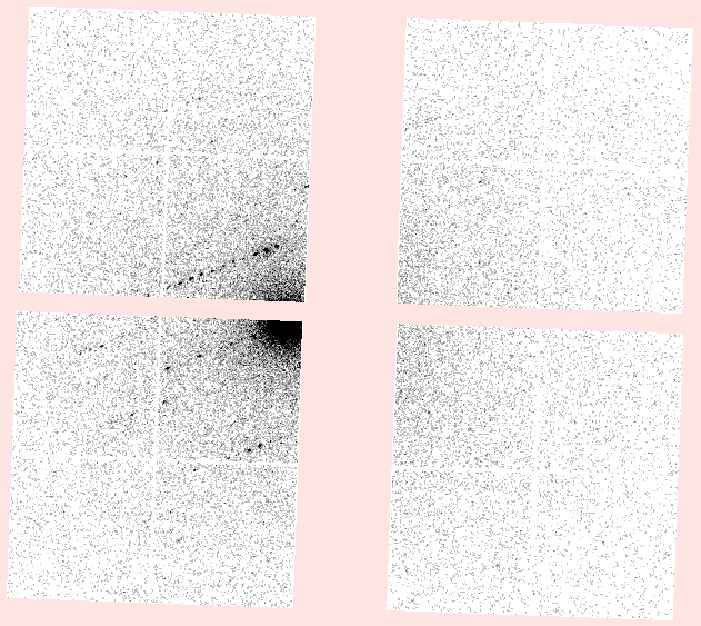
We did not allow the orientation of the rotation axis to refine, so errors in that will have been compensated by changes in the detector orientation. The dials.image_viewer displays the image as seen in the laboratory frame rather than the detector frame, so the image looks rotated. The fact that the detector “fast” and “slow” axes are no longer aligned with the laboratory X and -Y axes would not in itself negatively affect processing, but the fact that such large changes occurred during indexing meant we chose to repeat this process starting from the refined geometry. This can be done by re-importing the dataset using the refined geometry as a reference. On re-import, the site.phil files are no longer required, except for the oscillation which is not taken from the reference file. The import commands differ for each dataset as follows:

1. dials.import template=$DATA_PARENT/Lys_ED_Dataset_1/frame_value_###.cbf mask=mask.pickle \
     reference_geometry=refined_experiments.json geometry.scan.oscillation=0,0.076
   

2. dials.import template=$DATA_PARENT/Lys_ED_Dataset_2/frame_value_###.cbf \
     reference_geometry=refined_experiments.json geometry.scan.oscillation=0,0.1615 \
     lookup.dx=$DATA_PARENT/dx.pickle lookup.dy=$DATA_PARENT/dy.pickle
   

3. dials.import template=$DATA_PARENT/Lys_ED_Dataset_3/frame_value_###.cbf \
     reference_geometry=refined_experiments.json geometry.scan.oscillation=0,0.0344 \
     lookup.dx=$DATA_PARENT/dx.pickle lookup.dy=$DATA_PARENT/dy.pickle
   

4. dials.import template=$DATA_PARENT/Lys_ED_Dataset_4/frame_value_###.cbf \
     reference_geometry=refined_experiments.json geometry.scan.oscillation=0,0.0481 \
     lookup.dx=$DATA_PARENT/dx.pickle lookup.dy=$DATA_PARENT/dy.pickle
   

5. dials.import template=$DATA_PARENT/Lys_ED_Dataset_5/frame_value_###.cbf \
     reference_geometry=refined_experiments.json geometry.scan.oscillation=0,0.0481 \
     lookup.dx=$DATA_PARENT/dx.pickle lookup.dy=$DATA_PARENT/dy.pickle
   

6. dials.import template=$DATA_PARENT/Lys_ED_Dataset_6/frame_value_###.cbf mask=mask.pickle \
     reference_geometry=refined_experiments.json geometry.scan.oscillation=0,0.0481 \
     lookup.dx=$DATA_PARENT/dx.pickle lookup.dy=$DATA_PARENT/dy.pickle
   

7. dials.import template=$DATA_PARENT/Lys_ED_Dataset_7/frame_value_###.cbf \
     reference_geometry=refined_experiments.json geometry.scan.oscillation=0,0.0481 \
     lookup.dx=$DATA_PARENT/dx.pickle lookup.dy=$DATA_PARENT/dy.pickle
   

After re-importing with refined geometry, indexing and refinement of an orthorhombic solution was done as before.

Datasets 1-5 & 7

dials.index datablock.json strong.pickle refine.phil
dials.refine_bravais_settings indexed.pickle experiments.json refine.phil
dials.refine bravais_setting_5.json indexed.pickle refine.phil \
  output.experiments=static.json output.reflections=static.pickle

Dataset 6

Starting from the refined geometry, it was no longer necessary to fix the beam parameters or provide the unit cell for indexing. However, the unit cell restraint was still used.

dials.index datablock.json strong.pickle refine.phil restraint.phil
dials.refine_bravais_settings experiments.json indexed.pickle refine.phil
dials.refine bravais_setting_5.json indexed.pickle refine.phil restraint.phil \
  output.experiments=static.json output.reflections=static.pickle

Scan-varying refinement

Appropriate parameterisations for scan-varying refinement were determined as described in the publication.

Dataset 1

Varying beam, unit cell and crystal orientation:

dials.refine static.json static.pickle scan_varying=True \
  detector.fix=all \
  reflections.block_width=0.25 \
  beam.fix="all in_spindle_plane out_spindle_plane *wavelength" \
  beam.force_static=False \
  beam.smoother.absolute_num_intervals=1 \
  output.experiments=varying.json \
  output.reflections=varying.pickle

Dataset 2

Varying beam, unit cell and crystal orientation:

dials.refine static.json static.pickle scan_varying=True \
  detector.fix=all \
  reflections.block_width=0.25 \
  beam.fix="all in_spindle_plane out_spindle_plane *wavelength" \
  beam.force_static=False \
  output.experiments=varying.json \
  output.reflections=varying.pickle

Dataset 3

Varying beam and crystal orientation:

dials.refine static.json static.pickle scan_varying=True \
  detector.fix=all \
  reflections.block_width=0.25 \
  beam.fix="all in_spindle_plane out_spindle_plane *wavelength" \
  beam.force_static=False \
  crystal.unit_cell.force_static=True \
  output.experiments=varying.json \
  output.reflections=varying.pickle

Dataset 4

Varying crystal orientation:

dials.refine static.json static.pickle scan_varying=True \
  detector.fix=all \
  reflections.block_width=0.25 \
  beam.fix="all in_spindle_plane out_spindle_plane *wavelength" \
  crystal.unit_cell.force_static=True \
  output.experiments=varying.json \
  output.reflections=varying.pickle

Dataset 5

Varying crystal orientation:

dials.refine static.json static.pickle scan_varying=True \
  detector.fix=all \
  reflections.block_width=0.25 \
  beam.fix="all in_spindle_plane out_spindle_plane *wavelength" \
  output.experiments=varying.json \
  output.reflections=varying.pickle

Dataset 6

Varying beam and crystal orientation with static, restrained cell:

dials.refine static.json static.pickle scan_varying=True \
  detector.fix=all \
  reflections.block_width=0.25 \
  beam.fix="all in_spindle_plane out_spindle_plane *wavelength" \
  beam.force_static=False \
  crystal.unit_cell.force_static=True \
  restraint.phil \
  output.experiments=varying.json \
  output.reflections=varying.pickle

Dataset 7

Varying beam, unit cell and crystal orientation:

dials.refine static.json static.pickle scan_varying=True \
  detector.fix=all \
  reflections.block_width=0.25 \
  beam.fix="all in_spindle_plane out_spindle_plane *wavelength" \
  beam.force_static=False \
  output.experiments=varying.json \
  output.reflections=varying.pickle

Integration

Integration differed for each dataset by resolution limit, but otherwise used default parameters. After integration MTZs were exported for downstream processing with CCP4.

1. dials.integrate varying.json varying.pickle nproc=8 prediction.d_min=2.0
   dials.export integrated_experiments.json integrated.pickle mtz.hklout=integrated_1.mtz
   

2. dials.integrate varying.json varying.pickle nproc=8 prediction.d_min=2.3
   dials.export integrated_experiments.json integrated.pickle mtz.hklout=integrated_2.mtz
   

3. dials.integrate varying.json varying.pickle nproc=8 prediction.d_min=2.3
   dials.export integrated_experiments.json integrated.pickle mtz.hklout=integrated_3.mtz
   

4. dials.integrate varying.json varying.pickle nproc=8 prediction.d_min=2.2
   dials.export integrated_experiments.json integrated.pickle mtz.hklout=integrated_4.mtz
   

5. dials.integrate varying.json varying.pickle nproc=8 prediction.d_min=2.2
   dials.export integrated_experiments.json integrated.pickle mtz.hklout=integrated_5.mtz
   

6. dials.integrate varying.json varying.pickle nproc=8 prediction.d_min=2.5
   dials.export integrated_experiments.json integrated.pickle mtz.hklout=integrated_6.mtz
   

7. dials.integrate varying.json varying.pickle nproc=8 prediction.d_min=2.5
   dials.export integrated_experiments.json integrated.pickle mtz.hklout=integrated_7.mtz
   

Scaling and merging

The following commands assume the exported MTZs have been copied into a new directory together. Resolution limits were determined for each dataset individually, as described in the publication. These limits were then applied to the unscaled MTZs, while reindexing them to obtain the correct space group, \(P 2_1 2_1 2\):

declare -A RES
RES[1]=2.0
RES[2]=2.89
RES[3]=2.85
RES[4]=2.77
RES[5]=2.64
RES[6]=3.20
RES[7]=3.0

for i in {1..7}
do
  pointless hklin integrated_$i.mtz \
    hklout sorted_$i.mtz > pointless_reindex_$i.log <<+
RESOLUTION HIGH ${RES[$i]}
REINDEX L,-K,H
SPACEGROUP 18
+
done

The reindexed MTZs were combined and then scaled together with AIMLESS, setting an overall resolution limit of \(2.1 \unicode{x212B}\):

pointless hklin sorted_1.mtz \
          hklin sorted_2.mtz \
          hklin sorted_3.mtz \
          hklin sorted_4.mtz \
          hklin sorted_5.mtz \
          hklin sorted_6.mtz \
          hklin sorted_7.mtz \
    hklout combined.mtz > pointless_combine.log <<+
COPY
TOLERANCE 4
ALLOW OUTOFSEQUENCEFILES
+

aimless hklin combined.mtz hklout scaled.mtz > aimless.log <<+
resolution low 60 high 2.1
+

The scaled, merged MTZ is now ready for structure solution by molecular replacement.